Meetu Verma, Gal Matijevc, Carsten Denker, Andrea Diercke, Ekaterina Dineva, Horst Balthasar, Robert Kamlah, Ioannis Kontogiannis, Christoph Kuckein, Partha S. Pal
Leibniz-Institut für Astrophysik Potsdam AIP, Germany
As observational solar physicists, we collect copious amounts of data, especially high-resolution spectra. The number of spectra accumulated at a medium-size telescope (e.g., the Vacuum Tower Telescope, Tenerife) over one observing day easily reaches up to millions. Hence, we require tools to identify and classify spectra with minimal human intervention. Various machine learning techniques have been used in solar physics to classify or identify clusters in spectral data, however, employing t-distributed Stochastic Neighbor Embedding (t-SNE) is still very new. Our exploratory work provides the framework and some ideas on how to tailor the t-SNE classification scheme towards specific spectral data and well-defined science questions. Furthermore, we examined the choice of various t-SNE input parameters, the impact of seeing on classification, the results arising from various types of input data, and the link of the identified clusters to chromospheric features.
t-SNE as a Versatile Tool for Classifying Solar Spectra
t-SNE is a machine learning algorithm used for nonlinear dimensionality reduction [1]. In previous applications of t-SNE [2], it has proved to be a powerful tool for the initial selection of data, thus reducing their dimensionality. We applied t-SNE to high spectral resolution Hα contrast profiles. t-SNE projects these Hα profiles onto a two-dimensional map (Fig. 1). Although at first glance this map looks more like a point cloud, yet, using physical parameters to color code the point cloud, it becomes possible to recognize clusters. We used spectral line parameters computed using Cloud Model (CM) inversions to color code the t-SNE results. CM inversions allow to estimate physical parameters such as optical depth, Doppler width, line-of-sight velocity, and source function, which describe the properties of cool material suspended by magnetic fields in the chromosphere. The last map in Figure 1 shows that most of the Hα profiles which are suitable for CM inversions (green) are pushed to the periphery, whereas others are belonging to quiet Sun are concentrated more in the center (red).
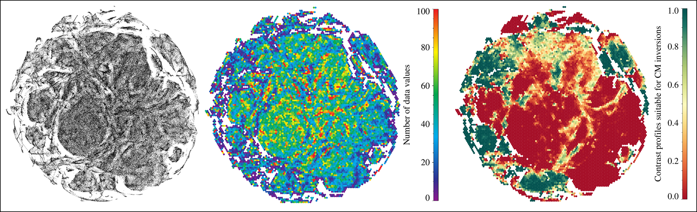
Figure 1. Two-dimensional t-SNE projection based on noise-stripped contrast profiles, appearing here as a ‘cloud’ of 415 800 individual data points (left). The number of contrast profiles per hexagonal bin (middle), i.e., a two-dimensional frequency distribution of the projection in the left panel, provides a visual guide to interpret the two-dimensional t-SNE projection. Contrast profiles suitable for CM inversions (green) are aggregated and projected into two dimensions based on t-SNE classification (middle) using hexagonal bins. Quiet-Sun and emission profiles (red) show low linear and rank-order correlations when comparing observed and CM-inverted contrast profiles.
From t-SNE Clusters to Feature Classes
As the initial results of t-SNE indicate, its strong discriminatory power arises from its ability to separate quiet-Sun and plage profiles from those that are suitable for CM inversions. As a demonstration, the ten largest clusters in the periphery are selected (left panel in Figure 2). These identified clusters are then back projected to the original observed scene on the solar surface. In an Hα slit-reconstructed image (middle panel of Figure 2), these cluster belong to dark regions with cool material, specifically tracing surges and filamentary structures [3]. Going one step further, we performed the t-SNE projection of the contrast profiles in these ten selected clusters (right panel of Figure 2) to see if the original clusters are preserved. As is evident from the figure, the original clusters are still present in the t-SNE projection.
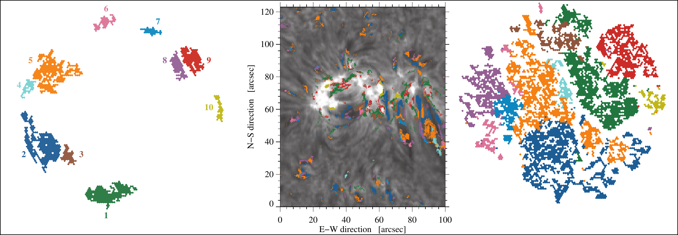
Figure 2. Clusters of Hα contrast profiles (left), which are suitable for CM inversions and which belong to the ten largest clusters in the two-dimensional histogram with hexagonal bins. The clusters are depicted in different colors and labeled by numbers. Back-projection of the ten clusters to the slit-reconstructed Hα line-core intensity image (middle) reveals their relationship to absorption features in the active region. Limiting the t-SNE input data to the back-projected contrast profiles yields a t-SNE projection that clearly preserves cluster membership (right).
In Figure 3, we compiled three hundred randomly selected contrast profiles for each of the ten clusters. In addition, average contrast profiles for each cluster are also displayed to identify characteristic profiles shapes. Similarities and differences in the profiles are clearly evident for the ten selected clusters. Some of these ten clusters can be aggregated to form classes. Combining the re-projected clusters in the right panel of Figure 2 with the spectral characteristics summarized in Figure 3 yields three classes: (1) Contrast profiles with a pronounced central component, i.e., Clusters 3, 1, 9, and 10 ordered according to increasing positive contrast. (2) Broad and deep profiles of Clusters 2 and 5, where the central maxima and neighboring minima exhibit similar amplitudes in contrast profiles. (3) Contrast profiles, where the central maximum is less pronounced and the contrast is almost everywhere negative, i.e., in Clusters 6, 7, and 8. Only the profiles of Cluster 4 cannot be clearly classified. Their location in the t-SNE projection (right panel of Figure 2) favors Class 2, whereas the predominantly negative contrast in Figure 3 suggests Class 3. Furthermore, these classes can be put in two categories with high (Class 1) and low (Classes 2 and 3) values of the source function. The distinction between Classes 2 and 3 is mainly due to differences in the cloud velocities, i.e., blue and redshifts of the spectral line. These three classes trace different absorption features. Class 1 profiles originate in the base of surges or arch filament structure, whereas Classes 2 and 3 trace the tip and middle part of surges.
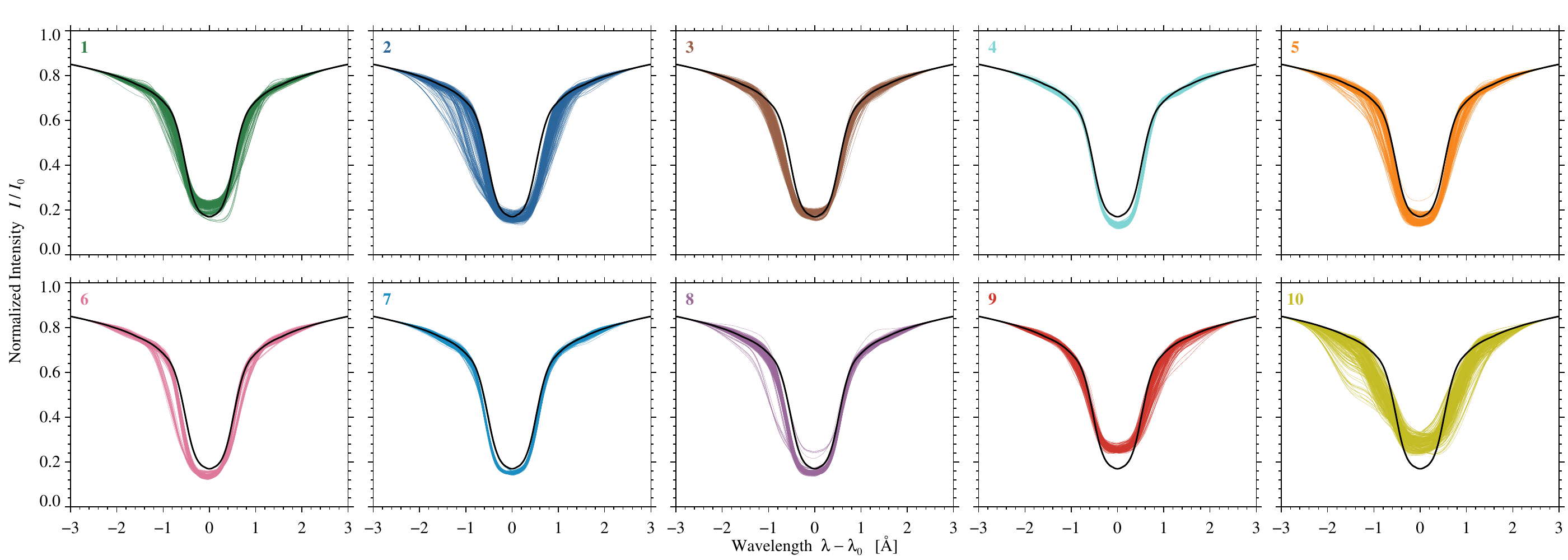
Figure 3. Three hundred randomly selected contrast profiles for the ten clusters of spectra. The color code is the same as in Figure 2. The average contrast profile (black-white dashed) for each cluster is plotted to capture the essential shape of the profile.
What’s Next?
The goal of this study was to establish a framework for classifying high-resolution spectra using t-SNE. Such a framework is particularly relevant in the context of Big Data ̶ not only because of the ease of its application but also because of the huge databases attached to solar research infrastructures. The new Daniel K. Inouye Solar Telescope (DKIST) and the upcoming European Solar Telescope (EST) will produce a plethora of data including high-spectral, spatial, and temporal resolution spectropolarimetric observations covering multiple spectral lines. Although t-SNE proves to be efficient in clustering high-dimensional data, human inference is still required at each step to interpret the results. This exploratory work establishes t-SNE as a suitable tool to cluster and classify high-resolution Hα spectra but also demonstrates that unsupervised machine learning algorithms provide the means to explore the ever-increasing data volume in solar spectroscopy.
References
[1] van der Maaten, L. & Hinton, G. 2008, J. Mach. Learn. Res. 9, 2579
[2] Matijevič, G., Chiappini, C., Grebel E. K., et al. 2017, Astron. Astrophys. 603, A19
[3] Verma M., Denker, C., Diercke, A., et al. 2020, Astron. Astrophys. 639, A19