R. J. Campbell, M. Mathioudakis, P. H. Keys, A. Reid, Chris Nelson (Queen's University of Belfast, Northern Ireland)
S. Shelyag (Deakin University, Australia)
C. Quintero Noda, Andrés Asensio Ramos, Manolo Collados (Instituto de Astrofísica de Canarias and Universidad de La Laguna, Spain)
David Kuridze (Aberystwyth University, UK)
The solar atmosphere is a magnetised plasma. Magnetic fields cause the light emitted from the Sun to become polarised. To observe these weak small-scale fields, we take advantage of the Zeeman effect, describing how spectral lines become split under the action of a magnetic field. At the centre of the solar disk, when the line of sight (LOS) and solar normal are aligned, measurement of Stokes I gives us the intensity, while Stokes Q and U (linear polarisation) and Stokes V (circular polarisation) reveals inclined and vertical fields, respectively. Constraining the magnetic vector’s inclination angle is a key goal, defined such that a value of 0 or 180 degrees represents a longitudinal (vertical, at disk centre) vector pointing towards or away from the observer, respectively, while 90 degrees represents a vector parallel to the solar surface. As instrumentation improves, attempts to infer the properties of the magnetic vector by analysis of the polarised light measured in observations of the solar photosphere continues to be fraught with risks, limitations, and challenges (see [1] for a full review).
Observing the dynamics of small-scale internetwork magnetic fields
Figure 1 shows a region of interest (ROI) with several magnetic features visible in the time-series of a scan of a disk centre quiet Sun internetwork (IN) region recorded on the 6 May 2019 [4] by the GREGOR Infrared Spectrograph Integral Field Unit (GRIS-IFU) instrument [2] at Europe’s largest solar telescope, GREGOR [3]. The large effective Landé g-factor and near infrared wavelength of the Fe I line at 1564.9 nm makes it an effective Zeeman diagnostic. This ROI includes a short-lived linear polarisation feature (LPF; red, dashed box in Fig. 1), a complex weak magnetic structure with mixed polarities and transverse fields (green, dotted box in Fig. 1) and a longitudinal kilo-Gauss magnetic element (upper right-hand side of Figure 1).
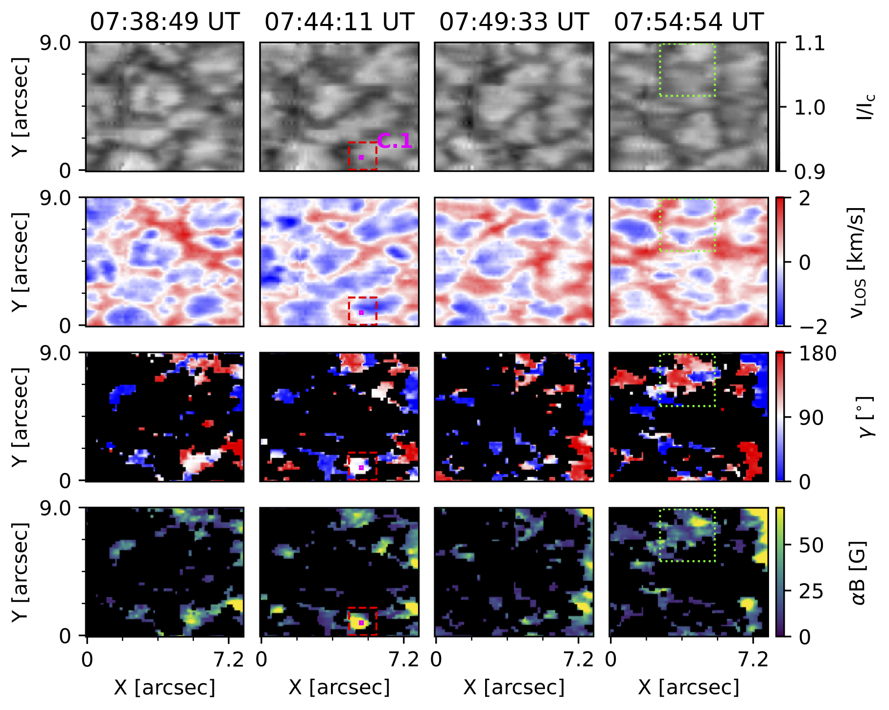
Figure 1 - Region of interest (ROI) observed in a GRIS-IFU scan showing maps of continuum intensity (top row) for a selection of frames (left to right). Parameters inferred from SIR inversions are shown, namely from top-bottom, line-of-sight velocity, inclination of the magnetic vector and magnetic flux density. Stokes I is normalised by the average continuum. Any Stokes parameter with maximum amplitude less than a noise threshold had been set to zero before inversion. Positive velocity values represent down-flows, and negative values represent up-flows. An inclination value of 0 degrees represents a vector pointing towards the observer, while 180 degrees indicates the opposite (from Campbell et al. 2021a).
By employing the Stokes Inversions based on Response functions code (SIR; [5]), we can infer the local thermodynamic, kinematic and magnetic properties of the atmosphere. Two-component models must be employed as we are not typically resolving the small-scale magnetic structures. We consider an inversion setup where a magnetic atmosphere is embedded in a field free medium. We therefore quantify the fraction of the pixel element occupied by the magnetic model using its filling factor, α.
Figure 2 shows a sample profile, labelled and marked as C.1 in Figure 1, from this LPF. The profiles have undergone a reconstruction process to remove noise and instrumental effects (see [4] for details). In the 1564.9 nm line, all lobes of Stokes Q and V are detected above the noise threshold, but Stokes U is not, and, thus, has been set to zero. We attempted to bin spatially around this pixel to lower the noise threshold, but the Stokes U profile still did not reach the threshold. Without the Stokes U profile, we do not have enough information to constrain the magnetic vector’s azimuthal angle, which defines the direction of the magnetic vector in the plane perpendicular to the observer’s LOS, but we can still infer its strength and inclination angle. Because the amplitude of Stokes Q is relatively large, one can infer that the magnetic field is clearly highly inclined but with a significant vertical component, and this is reflected in the inversion results. The weak field (B = 193 G) with large α (α = 0.761) is notable, resulting in a relatively large magnetic flux density (αB = 146 G).
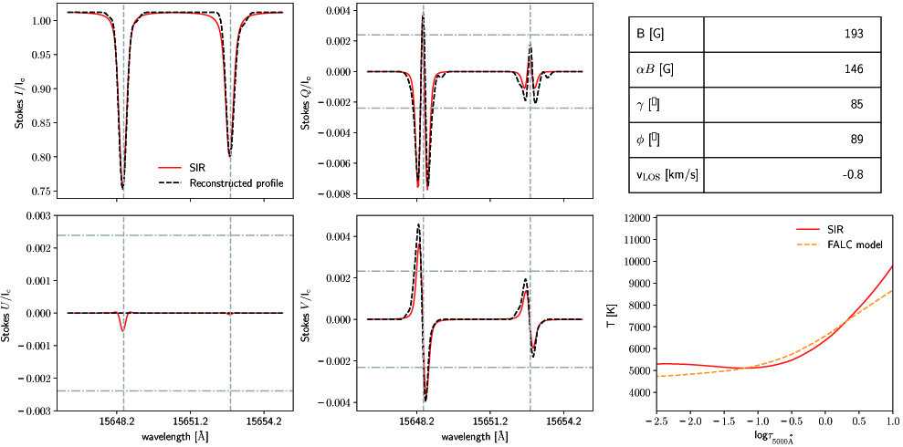
Figure 2 - Reconstructed full Stokes vector is shown for the 15648.52/15652.87 Å line pair in the left four panels, along with the synthetic profiles derived from the SIR inversions, for a sample profile. The horizontal (dot-dashed) lines show the noise thresholds for the polarised Stokes vectors, while the vertical (dashed) lines denote the rest wavelengths of each spectral line. On the right, the retrieved atmospheric parameters are shown in the table, namely (top-bottom) the unsigned magnetic field strength, magnetic flux density, inclination angle, azimuth angle and line of sight velocity . The temperature as a function of optical depth is shown in the lower right plot with the original input model. The magnetic parameters are from the magnetic model while the velocity is the combined value for both models (from Campbell et al. 2021a).
Comparison with magnetohydrodynamic simulations
One method for ensuring results derived from observations are well constrained is to compare them to realistic magnetohydrodynamic (MHD) simulations (e.g., [6]). In a new study (see [7] for pre-print), we use a snapshot of a realistic MURaM simulation ([8, 9]) to evaluate the extent to which we can retrieve accurate information about the magnetic vector in the IN photosphere using inversion techniques. We synthesize the full Stokes vector by solving the radiative transfer equation under the assumption of local thermodynamic equilibrium, only to then invert the synthetic spectra to establish the extent to which the original atmosphere differs according to the inversions. We then degrade the spectra to determine how they may have appeared had they been observed at the spatial and spectral resolutions achievable by GREGOR/GRIS-IFU.
Figure 3 shows a sample synthetic profile, located in a LPF similar to that shown in Fig. 1, degraded to GREGOR/GRIS-IFU resolutions along with the inversion results. Compared to the profile shown in Fig. 2, the magnetic field is also weak but relatively stronger (B = 337G) with smaller α (α = 0.425), resulting in a remarkably similar magnetic flux density (αB = 143 G).
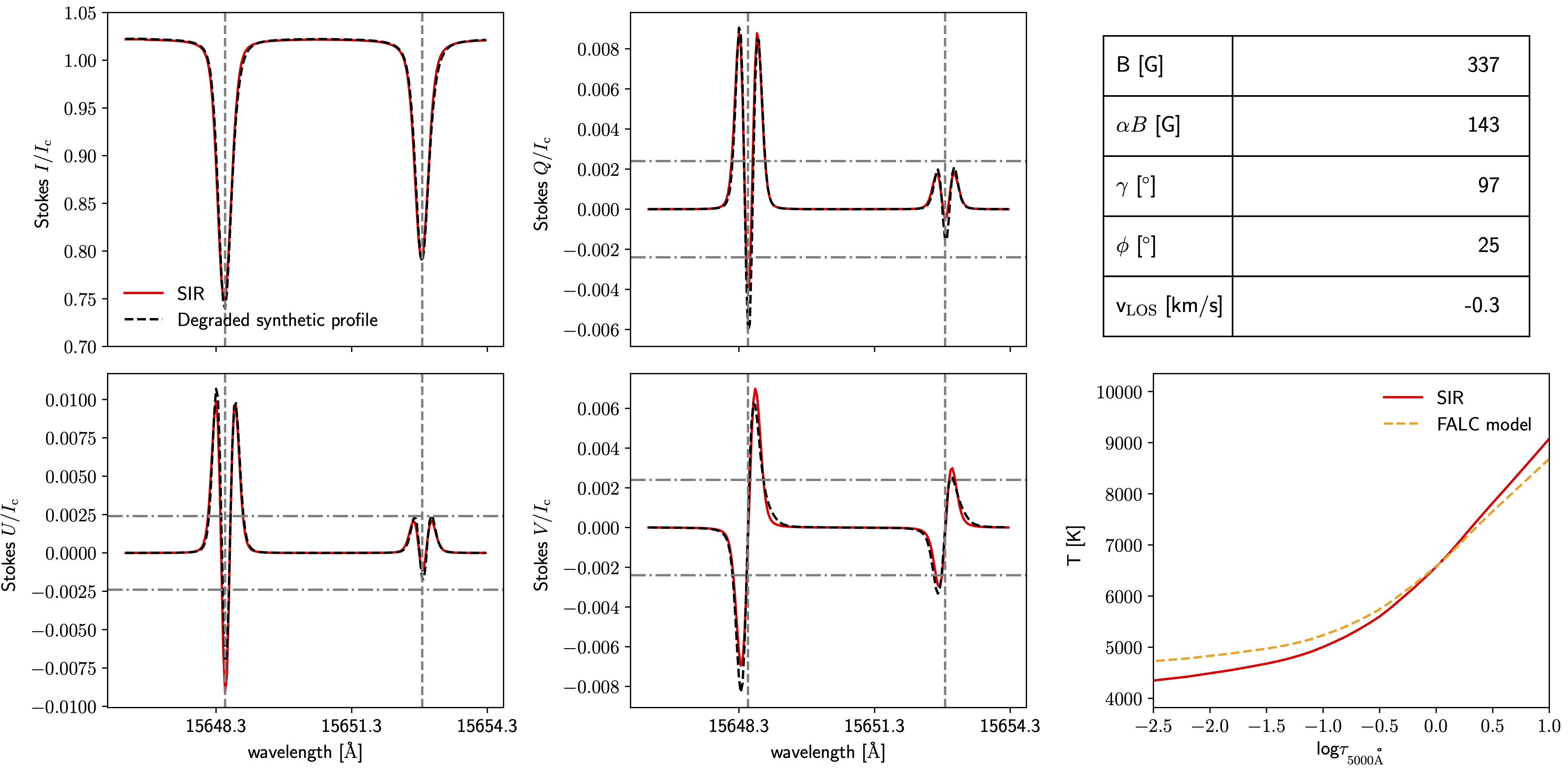
Figure 3 - As in Figure 2, except the full Stokes vector synthesised from realistic MHD (MURaM) simulation outputs after instrumental degradation (from Campbell et al. 2021b).
Next-generation solar telescopes
GREGOR can observe in this near infrared spectral window with an effective resolution of about 215 km. With higher spatial resolution, the measured polarisation signals will have a higher amplitude, as there will be less mixing of opposite polarities. Therefore, with the advent of next-generation high-resolution telescopes, like the Daniel K. Inouye Solar Telescope (DKIST; [10]) and the European Solar Telescope (EST), our understanding of how the magnetic field is organised in the IN photosphere is likely to experience a significant leap as observations reveal these regions of the solar atmosphere at unprecedented spatial resolution, with the simultaneous measurement of all four Stokes parameters in an increased number of pixels a key goal. The symbiosis between using MHD simulations as a guide in the interpretation of observations will continue to prove essential.
References
[1] – Bellot Rubio, L. & Orozco Suárez, D. 2019, Living Reviews in Solar Physics, 16, 1
[2] – Collados, M., López, R., Páez, E., et al. 2012, Astronomische Nachrichten, 333,872
[3] – Schmidt, W., von der Lühe, O., Volkmer, R., et al. 2012, Astronomische Nachrichten, 333, 796
[4] – R. J. Campbell, M. Mathioudakis, M. Collados, P. H. Keys, A. Asensio Ramos, C. J. Nelson, D. Kuridze and A. Reid, 2021a, A&A, 647 A182
[5] – Ruiz Cobo, B. & del Toro Iniesta, J. C. 1992, ApJ, 398, 375
[6] – Khomenko, E. & Collados, M. 2007, ApJ, 659, 1726
[7] – R. J. Campbell, S. Shelyag, C. Quintero Noda, M. Mathioudakis, P. H. Keys, and A. Reid, 2021b, under review with A&A (2021b)
[8] – Vögler, A., Shelyag, S., Schüssler, M., et al. 2005, A&A, 429, 335
[9] – Nelson, C. J., Shelyag, S., Mathioudakis, M., et al. 2013, ApJ, 779, 125
[10] – Rast, Mark P., Bello González, N., Bellot Rubio, L. and 87 others including R. J. Campbell, Critical Science Plan for the Daniel K. Inouye Solar Telescope (DKIST), 2021, Solar Physics, 296, 88 p., 70.
This research has received financial support from the European Union’s Horizon 2020 research and innovation program under grant agreement No. 824135 (SOLARNET).